Why Your T-Test Results Might Be Wrong: The Assumptions You're Probably Ignoring
When faced with a question like “Is surgery more expensive than therapy for fracture treatment?”, it’s tempting to jump straight into running a statistical test when we have the raw data ready. But as data scientists, we know that the most critical part of any analysis happens before we run the test. It’s in the careful validation of our assumptions.
In this post, I’ll walk you through how I approach a two-group comparison problem, emphasising the assumption-checking process that many practitioners skip. This isn’t just about getting the right answer. It’s about understanding why we can trust our results.
Setting Up the Problem
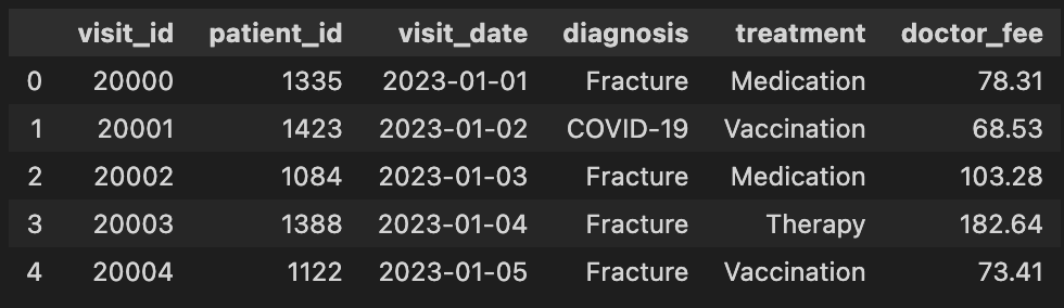
Our dataset contains patient treatment records with four types of diagnoses: COVID-19, FLU, Fracture, and Routine Checkup. Each diagnosis has multiple treatment options, and we’re interested in comparing doctor fees between different treatments.
The Research Question: For patients with fracture diagnoses, is surgery significantly more expensive than therapy?
This is a classic two-group comparison problem, which immediately suggests a t-test. But here’s where many analyses go wrong. They skip straight to the t-test without first asking: “Can we even use a t-test here?”
The Critical First Step: Isolating Your Variables
Before we can compare treatments, we need to control for confounding variables. Diagnosis type clearly affects doctor fees. A COVID-19 treatment will have different cost structures than a fracture treatment. To isolate the effect of treatment type on cost, we filter our dataset to focus only on fracture diagnoses.
This is a fundamental principle in data science: isolate the variables you want to study. By controlling for diagnosis type, we ensure that any differences we find are truly due to treatment choice, not diagnosis complexity.
Understanding T-Test Assumptions: Why They Matter
The t-test is a parametric test, meaning it makes specific assumptions about the underlying data distribution. These aren’t just academic requirements. They’re the foundation that makes the test valid. Violate them, and your p-values become meaningless.
The three key assumptions for a t-test are:
- Normality: The data in each group should be approximately normally distributed
- Independence: Observations should be independent of each other
- Equal Variance (for Student’s t-test): The two groups should have similar variances
Let’s address each one systematically.
Assumption 1: Checking for Normality
The normality assumption is often the most misunderstood. Many practitioners think they need perfectly normal data, but in practice, the t-test is reasonably robust to moderate deviations from normality, especially with larger sample sizes (typically n > 30).
However, we should still verify this assumption. Here’s my approach:
Visual Inspection First
Before running any statistical test, I always start with visualisation. Histograms with kernel density estimates give me an intuitive sense of the distribution shape. Are the distributions roughly bell-shaped? Are there obvious outliers or extreme skewness?
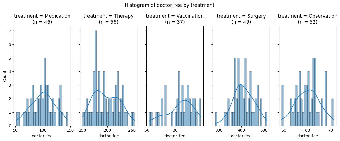
In our case, the visualisation show approximately normal distributions for all treatment groups, with sample sizes ranging from 37 to 56 patients per group. The distributions appear reasonably symmetric, which is a good sign.
Statistical Testing: Shapiro-Wilk Test
Visual inspection is subjective, so we complement it with a formal statistical test. The Shapiro-Wilk test is one of the most powerful tests for normality, especially for smaller sample sizes.
The test works by comparing our data’s distribution to a perfect normal distribution. If the p-value is greater than our significance level (typically 0.05), we fail to reject the null hypothesis that the data is normally distributed.
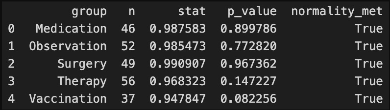
For all treatment groups in our analysis, the Shapiro-Wilk test returned p-values well above 0.05, confirming that we cannot reject the normality assumption. This is particularly important for the two groups we’re comparing: Surgery (p = 0.967) and Therapy (p = 0.147).
Key Takeaway: Always use both visual and statistical methods to assess normality. Visual inspection catches obvious problems, while statistical tests provide objective validation.
Assumption 2: Independence
The independence assumption means that each observation should be independent of others. In our case, this means one patient’s treatment cost shouldn’t influence another patient’s cost. This is typically satisfied when we have a random sample, which we assume here.
This assumption is usually assessed through study design rather than statistical testing. We need to ensure our data collection method didn’t introduce dependencies.
Assumption 3: Equal Variance (Homogeneity of Variance)
This assumption determines which type of t-test we should use:
- Student’s t-test: Assumes equal variances between groups
- Welch’s t-test: Does not assume equal variances (more robust)
We test this using Levene’s test, which compares the variances of our two groups. If the p-value is greater than 0.05, we assume equal variances and can use Student’s t-test. Otherwise, we use Welch’s t-test.
if normality_met and equal_variance:
    test_used = "student_t"
    equal_var_flag = True
else:
    test_used = "welch_t"
    equal_var_flag = False   # Welch does not assume equal variances
Formulating the Hypothesis
Now that we’ve validated our assumptions, we can proceed with hypothesis testing. But first, we need to clearly state what we’re testing.
Null Hypothesis (H₀): Surgery, on average, does not have a higher price compared to therapy. Any observed difference is due to random variation.
Alternative Hypothesis (H₁): Surgery, on average, does have a higher price compared to therapy, and this difference is not due to random variance.
Notice that we’re using a one-sided test (alternative=”greater”) because we’re specifically testing whether surgery is more expensive, not just different. This is more powerful than a two-sided test when we have a directional hypothesis, but it requires that we’re confident in the direction before looking at the data.
Running the Test: The Easy Part
Once we’ve done all the assumption checking, running the actual t-test is straightforward. Our automated function checks normality and variance, then selects the appropriate test (Student’s or Welch’s) and runs it.
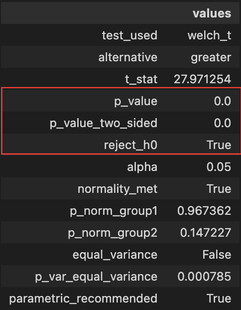
The results show that surgery is significantly more expensive than therapy (p < 0.05), allowing us to reject the null hypothesis.
Beyond Statistical Significance: Practical Significance
Statistical significance tells us that the difference is unlikely due to chance, but it doesn’t tell us if the difference matters in practice. That’s where practical significance comes in.
In our analysis, surgery is approximately 2.1× more expensive than therapy. This is a substantial difference that has real-world implications for patients and healthcare decision-makers.
We also examine the coefficient of variation to understand the relative variability in costs across treatments, which helps contextualise the cost differences.
coefficient_variation = df.groupby("treatment")["doctor_fee"].agg(["mean", "std"])
coefficient_variation["cv"] = coefficient_variation["std"] / coefficient_variation["mean"]
The Data Scientist’s Mindset
What I hope you take away from this analysis isn’t just the specific steps, but the mindset:
-
Never skip assumption checking. It’s not optional. It’s what makes your analysis valid.
-
Use multiple methods. Visual inspection and statistical tests complement each other. Don’t rely on just one.
-
Understand what you’re testing. Know the difference between one-sided and two-sided tests, and choose based on your research question.
-
Consider practical significance. A statistically significant result might not be practically meaningful.
-
Automate the process. Build functions that check assumptions automatically. This reduces errors and makes your analysis reproducible.
Conclusion
The t-test itself is simple to run. Just a few lines of code. But the real work happens in the assumption checking phase. By systematically validating normality, independence, and variance assumptions, we ensure that our statistical conclusions are trustworthy.
In our case, we found that surgery is indeed significantly more expensive than therapy for fracture treatment. Approximately 2.1× more expensive on average. But more importantly, we can be confident in this conclusion because we validated the assumptions that make the t-test appropriate for our data.
The next time you’re tempted to run a t-test immediately, pause and ask yourself: “Have I checked my assumptions?” Your future self (and your readers) will thank you.
All the code can be checked on my GitHub: https://github.com/ygcahyono/ds_personal_logging/blob/main/20251128-ab-testing-statistical-significance/002-lab-ttest.ipynb_